Plotting Examples
We have included a few functions to generate plots of CHAMP domains and resolution parameter estimates in the singlelayer and multilayer cases. We encourage you to make your own application-specific plotting code as well (the source code in modularitypruning.plotting is very straightforward and may provide inspiration).
Plotting Single-Layer CHAMP Domains and Resolution Parameter Estimates
- plot_estimates(gamma_estimates)
Plot partition dominance ranges with gamma estimates.
- Parameters:
gamma_estimates – gamma estimates as returned from
ranges_to_gamma_estimates()
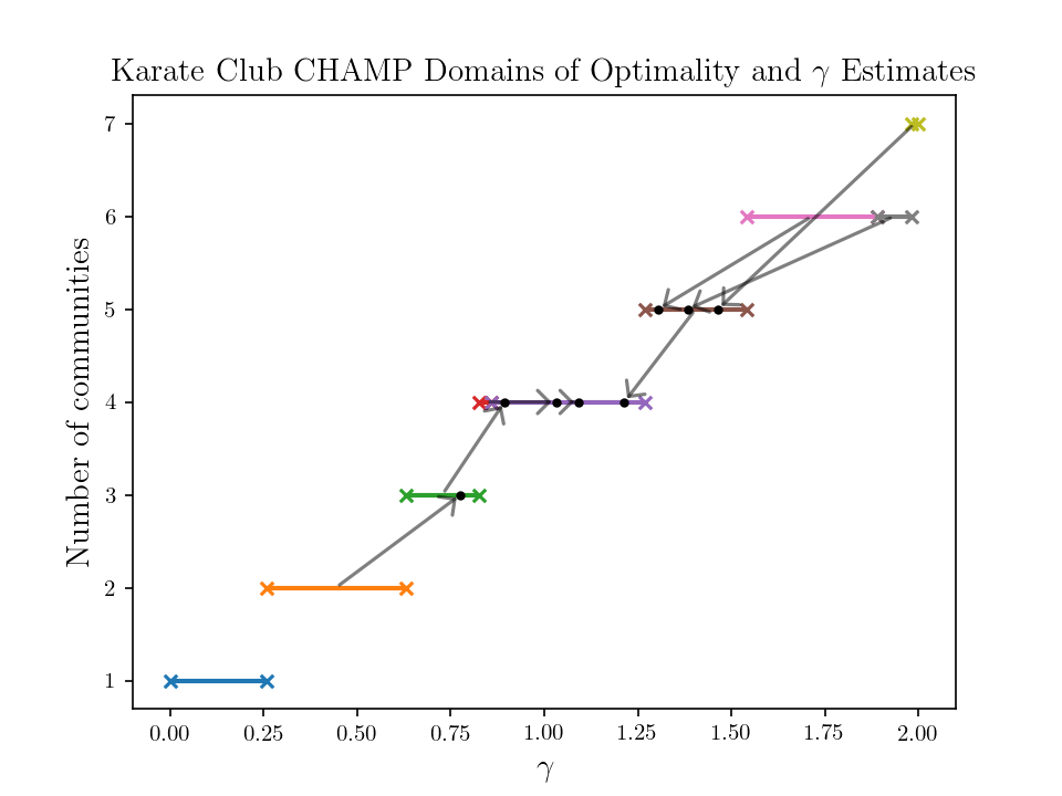
An example on the Karate Club network is as follows.
import igraph as ig
import matplotlib.pyplot as plt
from modularitypruning.champ_utilities import CHAMP_2D
from modularitypruning.parameter_estimation_utilities import ranges_to_gamma_estimates
from modularitypruning.leiden_utilities import repeated_parallel_leiden_from_gammas
from modularitypruning.plotting import plot_estimates
import numpy as np

# get Karate Club graph in igraph
G = ig.Graph.Famous("Zachary")

# run leiden 100K times on this graph from gamma=0 to gamma=2 (takes ~2-3 seconds)
partitions = repeated_parallel_leiden_from_gammas(G, np.linspace(0, 2, 10 ** 5))

# run CHAMP to obtain the dominant partitions along with their regions of optimality
ranges = CHAMP_2D(G, partitions, gamma_0=0.0, gamma_f=2.0)

# append gamma estimate for each dominant partition onto the CHAMP domains
gamma_estimates = ranges_to_gamma_estimates(G, ranges)

# plot gamma estimates and domains of optimality
plt.rc('text', usetex=True)
plt.rc('font', family='serif')
plot_estimates(gamma_estimates)
plt.title(r"Karate Club CHAMP Domains of Optimality and $\gamma$ Estimates", fontsize=14)
plt.xlabel(r"$\gamma$", fontsize=14)
plt.ylabel("Number of communities", fontsize=14)
plt.show()
which generates
Plotting Multi-Layer CHAMP domains and Resolution Parameter Estimates
- plot_2d_domains_with_estimates(domains_with_estimates, xlim, ylim, plot_estimate_points=True, flip_axes=True)
Plot partition dominance ranges in the (gamma, omega) plane, using the domains from CHAMP_3D with their gamma and omega estimates overlaid.
Limits output to xlim and ylim dimensions. Note that the plotting here has x=omega and y=gamma.
- Parameters:
domains_with_estimates – CHAMP domains and resolution parameter estimates as returned from
domains_to_gamma_omega_estimates().xlim – plotting x limits
ylim – plotting y limits
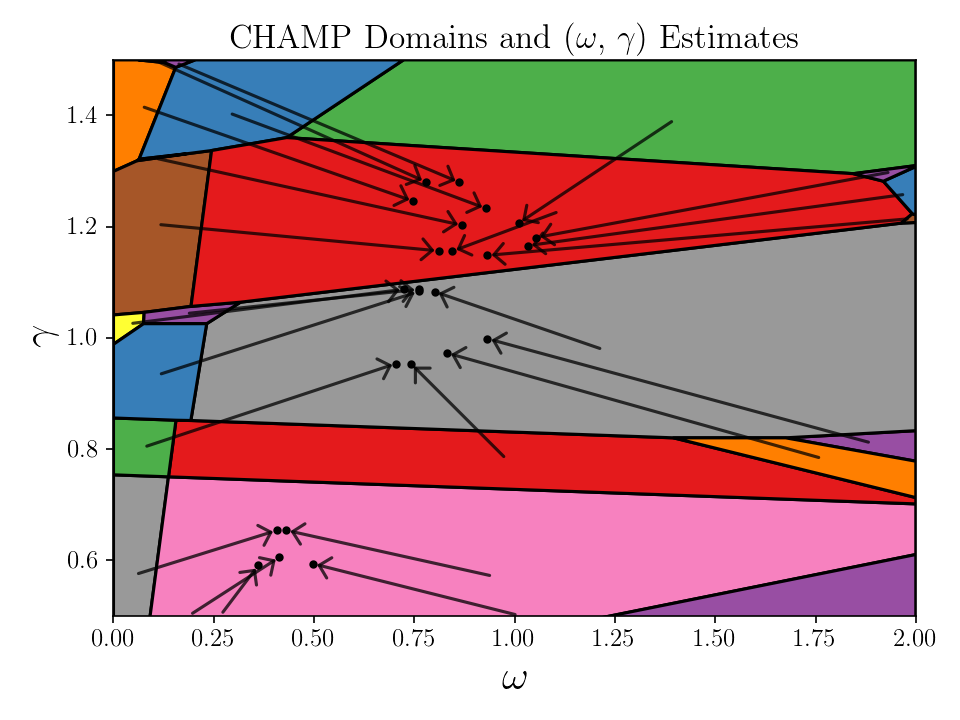
An example on a realization of multilayer synthetic network in Basic Multilayer Example is as follows.
from modularitypruning.champ_utilities import CHAMP_3D
from modularitypruning.leiden_utilities import repeated_parallel_leiden_from_gammas_omegas
from modularitypruning.parameter_estimation_utilities import domains_to_gamma_omega_estimates
from modularitypruning.plotting import plot_2d_domains_with_estimates
import matplotlib.pyplot as plt
import numpy as np

# run leiden on a uniform grid (10K samples) of gamma and omega (takes ~3 seconds)
gamma_range = (0.5, 1.5)
omega_range = (0, 2)
parts = repeated_parallel_leiden_from_gammas_omegas(G_intralayer, G_interlayer, layer_vec,
                                                    gammas=np.linspace(*gamma_range, 100),
                                                    omegas=np.linspace(*omega_range, 100))

# run CHAMP to obtain the dominant partitions along with their regions of optimality
domains = CHAMP_3D(G_intralayer, G_interlayer, layer_vec, parts,
                   gamma_0=gamma_range[0], gamma_f=gamma_range[1],
                   omega_0=omega_range[0], omega_f=omega_range[1])

# append resolution parameter estimates for each dominant partition onto the CHAMP domains
domains_with_estimates = domains_to_gamma_omega_estimates(G_intralayer, G_interlayer, layer_vec,
                                                          domains, model='temporal')

# plot resolution parameter estimates and domains of optimality
plt.rc('text', usetex=True)
plt.rc('font', family='serif')
plot_2d_domains_with_estimates(domains_with_estimates, xlim=omega_range, ylim=gamma_range)
plt.title(r"CHAMP Domains and ($\omega$, $\gamma$) Estimates", fontsize=16)
plt.xlabel(r"$\omega$", fontsize=20)
plt.ylabel(r"$\gamma$", fontsize=20)
plt.gca().tick_params(axis='both', labelsize=12)
plt.tight_layout()
plt.show()
which generates
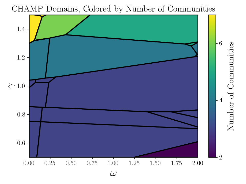
- There are other similar functions
plot_2d_domains()essentially plots the above without arrows showing resolution parameter estimatesplot_2d_domains_with_ami()plots CHAMP domains, colored by the AMI between each partition and a ground truthplot_2d_domains_with_num_communities()plots CHAMP domains, colored by number of communities
For example, the last function generates
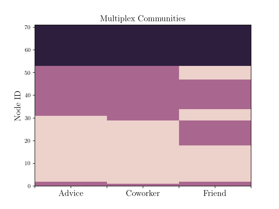
Plotting Multiplex Community Structure of a Single Partition
- plot_multiplex_community(membership, layer_vec)
Plot a visualization of multiplex community membership
- Parameters:
membership (tuple[int]) – partition membership vector
layer_vec (list[int]) – list of each vertex’s layer membership
An example from the Lazega Law Firm network is as follows
from modularitypruning.plotting import plot_multiplex_community
import matplotlib.pyplot as plt
import numpy as np

num_layers = 3
layer_vec = [i // 71 for i in range(num_layers * 71)]
membership = [1, 1, 0, 0, 0, 0, 0, 0, 0, 0, 0, 0, 0, 0, 0, 0, 0, 0, 0, 0, 0, 0, 0, 0, 0, 0, 0, 0, 0, 0, 0, 1, 1, 1, 1,
              1, 1, 1, 1, 1, 1, 1, 1, 1, 1, 1, 1, 1, 1, 1, 1, 1, 1, 2, 2, 2, 2, 2, 2, 2, 2, 2, 2, 2, 2, 2, 2, 2, 2, 2,
              2, 1, 0, 0, 0, 0, 0, 0, 0, 0, 0, 0, 0, 0, 0, 0, 0, 0, 0, 0, 0, 0, 0, 0, 0, 0, 0, 0, 0, 0, 1, 1, 1, 1, 1,
              1, 1, 1, 1, 1, 1, 1, 1, 1, 1, 1, 1, 1, 1, 1, 1, 1, 1, 1, 2, 2, 2, 2, 2, 2, 2, 2, 2, 2, 2, 2, 2, 2, 2, 2,
              2, 2, 1, 1, 0, 0, 0, 0, 0, 0, 0, 0, 0, 0, 0, 0, 0, 0, 0, 0, 1, 1, 1, 1, 1, 1, 1, 1, 1, 1, 1, 0, 0, 0, 0,
              0, 1, 1, 1, 1, 1, 1, 1, 1, 1, 1, 1, 1, 1, 0, 0, 0, 0, 0, 0, 2, 2, 2, 2, 2, 2, 2, 2, 2, 2, 2, 2, 2, 2, 2,
              2, 2, 2]

plt.rc('text', usetex=True)
plt.rc('font', family='serif')
ax = plot_multiplex_community(np.array(membership), np.array(layer_vec))
ax.set_xticks(np.linspace(0, num_layers, 2 * num_layers + 1))
ax.set_xticklabels(["", "Advice", "", "Coworker", "", "Friend", ""], fontsize=14)
plt.title(f"Multiplex Communities", fontsize=14)
plt.ylabel("Node ID", fontsize=14)
plt.show()
which generates